Atmospheric physics

This study try to describe the atmospheric phenomena, so what is happening under the atmospheric boundary layer? In this layer when there are orographic and urban effect, mathematics simulator models, air diffusion of pollution and estimation of energy resources.

To analyze the physics effect in the Earth is necessary to know the real situation thank the use of different scale about spatial and temporal visions.

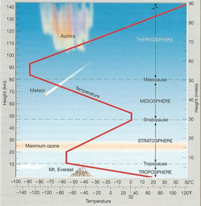
In the image in right we can see the vertical structure of atmosphere, from soil to 150 km in the thermosphere. It's represented the variation of temperature with the height and the most famous phenomena in the sky.

An important element in the air is the ozone O3 which works like a barrier for UV ray and thermal effects of the soil.

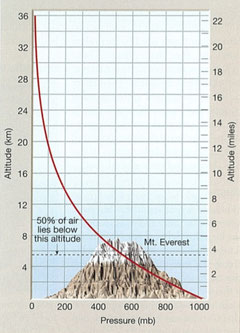
A very important relation is the Stevin Law which explains the variation of pressure p with the height z.

This relationship decreases with the factor between the density of air and the gravitational acceleration g. In effect, on the soil (z = 0 m) there is maximum of pressure, while on the 30 km of height there is about 0 hPa. The medium value of pressure is reported between 6 km of height, to the decreasing is like exponential law. On the zero level is reported a pressure medium between 1013 hPa.

For studying the atmospheric thermodynamic is necessary to know some parameters which describe temperature, pressure and volume with the energy by work and heat. The pseudo-adiabatic chart is an example of relationships between some parameters, to found an unknown value.

With these characteristics, it's possible to determining some boundary layer in the atmosphere:

- lifting condensation level (LCL),

- level of free convection (LFC),

- convective available potential energy (CAPE),

- equilibrium level (EL).

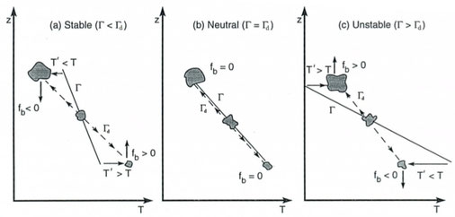
Now is possible to defining stability condition and instability condition by the relation between different adiabatic gradient.

The first graphic put a dry adiabatic gradient greater then real temperature gradient: a particle converges because the colder particle is heaviest. So this is a description of stability condition of atmosphere, with less heat variation and phenomena.
The second graphic put a dry adiabatic gradient lower then real temperature gradient: a particle diverges because it's hotter the a real particle and go upper. So this is a description of instability condition, when we can see lot of heat exchange and great phenomena like rain.

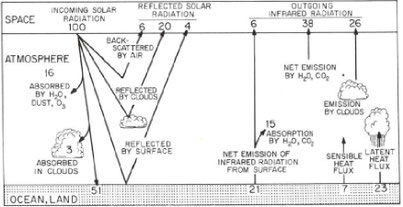
Another aspect of atmosphere is the Solar radiation, so how much and what type of Solar ray arrives in Earth soil? And what are the effects?

That is depending by the air chemical composition, so how many hydrogen, oxygen and carbon are in the atmospheric gas.

For this analyse is necessary to know the electromagnetic aspect of Solar ray with the Plank law, so it's important describe the UV effects and the IR effects; how much ray can go beyond the atmosphere? There are some studies which explain the percentages of radiation in the Earth, with a thermodynamic vision about the gas effects.

The first studio to understanding the atmospheric condition is by motions on a synoptic scale; so the definition of Navier-Stokes relationship when we can improve the balances of energy and mass. There is the usual problem of fluid mechanics: the close law for determining the system.

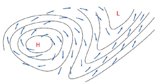
The image in the right is the result of relation between height and low pressure zones with the wind deviation by the local effects. In general the wind go along the isobaric lines, like clockwise in H and counterclockwise in L, but in synoptic scale we can see a little angle of divergent in H and convergent in L.

It's defined a Rossby number like a relation between inertial term and Coriolis effect, to defining the deviation angle.

In terms of synoptic scale, there is the difference between absolute vorticity and relative vorticity. Of course, absolute vorticity is the sum of relative and terrestrial vorticity f.

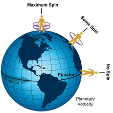
So the variation of absolute vorticity is depending by 3 physic characteristics:

- stretching

- tilting

- solenoidal

These parameters describe Earth form and the image a the right is the physical demonstration, how change spin in different part of the Earth.

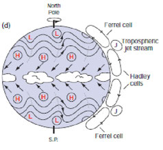
By vorticity theory is made the cyclogenesis theory, which explains the jet stream ripple on the atmosphere.

The Rossby waves are the variation of these winds between low and high pressure in Ferrel cell and Hadley cell. That phenomena is the base of cold and hot fronts, so the causes of bad weather and atmospheric phenomena.

It's necessary to remember the hot air is lighter than cold air, so when an hot front is arriving it goes on and it makes diffused clouds; but when a cold front is arriving it goes down and it makes piles of clouds with possibility of rain.

The cold air is faster than hot front, so is the fronts meet a storm is generated.

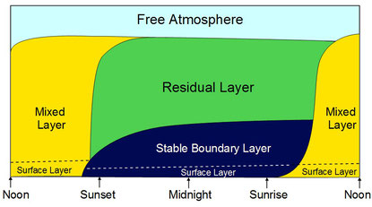
The Atmospheric boundary limit is a part of Troposphere which is influenced by soil surface.

Its depth changes according to environmental conditions as: climate, hours, season and type of soil; it changes between some meters for stability conditions to one kilometers for instability conditions.

In the picture of right page, we can see how atmosphere is composed and how it changes in a day.

So there, in surface layer, it's necessary to calculate turbulence phenomena through balance equations. We have got an indeterminate system which is closed by turbulent diffusion.

In that atmospheric zone, there is the Ekman boundary limit: where the cross wind v is zero; the height is about [pi greek/gamma], so is depending by mixed layer parameters.

Another significant height will be the convective boundary layer (CBL), that is the separation line between mixed layer and free atmosphere entrainment zone.

FIRST CASE: Sea Breeze

The water system has got an higher thermal capacity than soil system; therefore, on the night water of sea is hotter than ground, so there is a light wind from land to the sea. During the day, the Sun heats the coast, so the water is colder than the ground and there is a light wind from sea to land.

On day this wind can take some cloud at top of cycle.

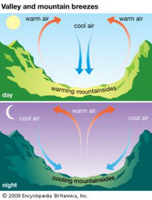
SECOND CASE: Valley Wind

During the day, the Sun can heats slope in different way, before the top of a mountain on sunrise, than on valley. So there, on a day there is hotter wind to top of the slope and colder wind downs on center of valley. On the night, there is inverse system and on slope we can see colder wind downs to valley.

This wind system is the same between a valley and a flat land: during the day, wind came from plain to valley (up-valley), vice versa on the night (down-valley).

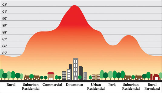
A heat island effect is the consequence of a great urban land, where there is a great difference of temperature between urban center and country around the city.

The major causes are absorption of heat on city, perspiration and evaporation on country and water penetration of permeable soil. The maximum intensity of heat is on night, when the difference of temperature is highest, about 10 degrees.

The Cliff phenomena is on boundary between urban land and country, its intensity is calculated as the difference of temperature between a point of urban land and another point outside.

So this assessment is possible though the Heating Degree Day (HDD), it is defined as heat requirements of a build. The same assessment is made with Cooling Degree Day (CDD) calculation.

For several sanity problems it's necessary to mitigate these effects on urban center, so it will be good solution increase the green soil onside the city, with trees or gardens. On this way, the difference of temperature will be reduced and the well-being will increase.