
Fluvial engineering
REQUIRES:
fluid mechanics
hydrodynamic
hydrology
VIA
building technical
geotechnical
math analysis
CONTENTS:
natural algae roughness
sediments
classification
movement, transportation
mathematics models
works
It is necessary to establish a relation between the flow of a water course and its tie.
To improve this operation, it has to know characteristics of the fund, with a value of roughness.
The study is not immediate and it is never exact; but there are many methods to calculating a right value of this aspect.
The first aspect which is observed is the mobile or fixed fund.
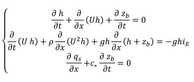
Equilibrium equations
MASS BALANCE:
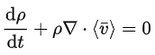
From hydrodynamic studies we can analyse the mass balance of a small infinitesimal element to respecting the mass conservation. So the mass of fluid which enter to the control volume will be equal of the mass of fluid which exit, with the assumption of incompressible fluid.
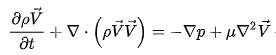
BALANCE OF THE MOMENTUM:
By the Reynolds studies of the turbulence effects, it is possible to "close" the indeterminate problem.
It is necessary to defining the state of fluid to determine the tension to the wall: there some difference between smooth wall and rough wall, but there is always a logarithmic law to identify these parameters.
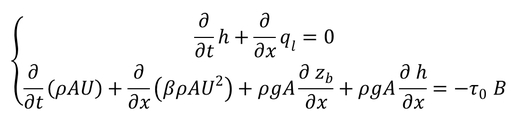
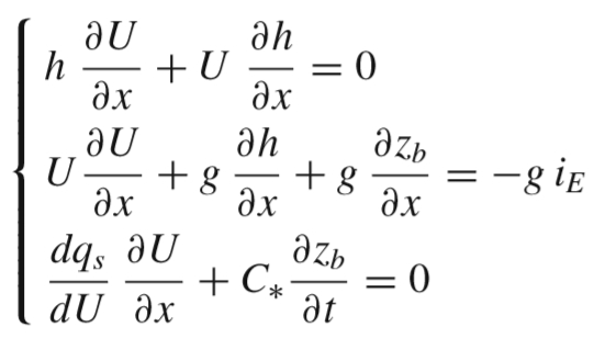
Therefore, to complete the river study, it is possible to approximate the depth and having the general system of balance equations. On right we can see the structure of system, which will be integrated with close relation and boundary conditions.
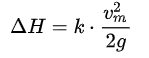
Most important relation to resolve these system problem can be the Darcy - Weisbach equation, with the kinetic term.
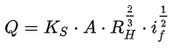
Another relation which use to know water flow is the Gauckler - Strickler equation with the roughness value of fund.
Sediments
There are 5 major problems to determine a real roughness value:
1. maximum speed
2. low submergence
3. vegetation
4. non-compact sections
5. non-uniform roughness
Problem 1
The Boussinesq diffusive model for turbulent state explains that the point of maximum speed is in the center of section, away the lateral walls. Looking for vertical axis, there is a parabolic law which put zero speed on surface and bottom sites. The maximum value of speed is down water surface, about a quarter of depth.
Problem 2
The case of low submergence is look like in mountain torrents, with low depth and high inclination, rough and heterogeneous bottom.
There are different relations of speed, with both terms of average and fluctuations. The distribution of speed is a logarithmic law (Nikora rational formula) or there are empirical relations which describe the distribution with a power law. These formula are based on constants tabulated by English scholar and USGS corp. Best solution is by Meyer-Peter & Muller with a power law of roughness from granulometry analysis.
Problem 3
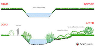
Vegetation is classified in three types: herbaceous, shrubby and arboreal vegetation.
First one is always under water, flexible and plastic; in this case Ks coefficient is like height of vegetation, and the effect is minimum if depth is much greater than the height.
Second one is always under water, partially flexible and elastic; in this case we can use the Kowen & Unny method through some parameters of vegetation like.
Third one is emerging, rigid and regularly distributed; in this case we have to consider equivalent coefficient of roughness with different point of river section, we are considering the trees form and geometry to improve vegetation parameters in the formula.
Problem 4
If the section presents some floodplains, the bottom is not homogeneous and it's defined non-compact. So that it's necessary to study the different parts of section and sum it. There some techniques for result value, but the most reliable is Lotter method, with a weighted average.
The latter semplification involves a margin of error, in that this condition occurs only on the lines normal to isotachs; therefore it it these lines which should be used to subdivide the cross section. If the horizontal width of subareas is much greater than the water depth, any possible error is rather modest.
Problem 5
Last problem is about mixed roughness, so it's necessary to calculate a weighted average of rough coefficient with the Einstein-Horton formula which is depending by the wet outline of section.
Therefore sediments are classified in different way: by dimension, form and density.
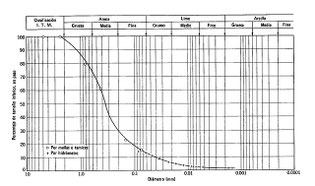
The dimension is calculated with diameter analysis in the granulometry through sediment sifter. There are three way to measure form of sediments. Different diameters makes different classes, so there is the Udden Went Worth classification which lists: boulders, shingle, gravel, sand, silt and clay (from coarse grain to fine-grained). Finally, with a concentration analysis of a control volume, we can define some density classes.
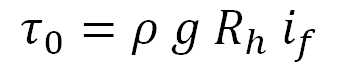
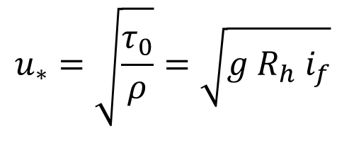
An other important issue is about the friction of the bottom. This part consists on determination of close relation and parameter TAU. It depends by angle and wet contour, and then it is possible to calculate a friction speed by the next radical formula.
So, these parameters permit to complete the mathematical study of flow, with the variables: water speed, depth and erosion effects.
Incipient motion
Sediments can be in bottom if they are coarse grain or in suspension if they are fine-grained.
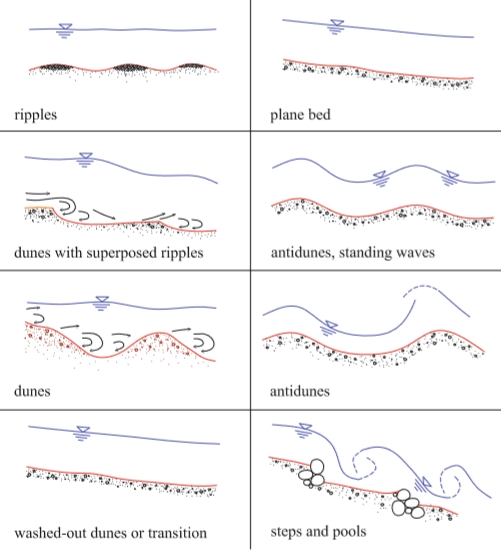
There are five regimes for divide behavior of the channel:
1. plane beds;
2. small ripples;
3. channel with dunes which move to valley;
4. transcritical condition;
5. channel with dunes which move to mount.
The study of incipient motion is based by two approaches:
- deterministic way, with temporal average;
- probabilistic way, with turbulence fluctuations.
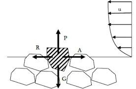
The Shields approach assumes large section, horizontal bottom, homogeneous and stationary motion and homogeneous materials.
In the image we can see forces at stake. So G represents gravity weight, A represents acceleration, P is the lift and R is the bottom resistance for the roughness. There is incipient motion when the resistance is less than acceleration.
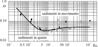
Shields approach takes a logarithmic diagram which explain three terms; so there is line relation of critical condition of incipient motion and two zones: of solid transportation (over line) and no solid transportation (under line).
Therefore it is necessary to define the critical parameter by sediments definition. Some studies are been by Shields, Bonnefille and Parker to find best critical relation with transportation condition. In general, for high value of Reynolds, critical coefficient is about 0.06.
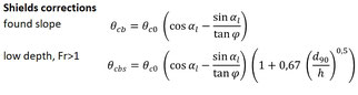
These assessments need the effects of hideing, curve and static armouring with some corrections on the original formula.
For this effects, it study a found motion in function of flow behaviors. Though the distribution of stresses, we can assess the flow with H.A.Einstein method, Meyer-Peter & Muller and Engelund method or Van Rijn method.
Solid transport is classified in rolling, jumping, suspension and runoff in function of flow and diameter of materials.
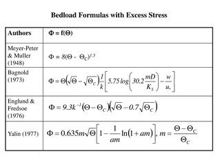
On right of this page, there is the comparison of Stress formulas by MPM, Bagnold, Engelund & Fredsoe and Yalin, when dimensionless flow is on function of Shields parameter.
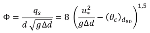
In conclusion, this is Meyer-Peter & Muller formula for the definition of Shields parameter. It can explain the relationship between solid flow and critical status through friction speed on the bottom.
The transport in found
H. A. Einstein introduced some hypothesis in him theory of materials flow: homogeneous and stationary motion, homogeneous materials and constant range.
Einstein can calculate the probability of crossing of a solid element across a general section A from a general side on the bottom.
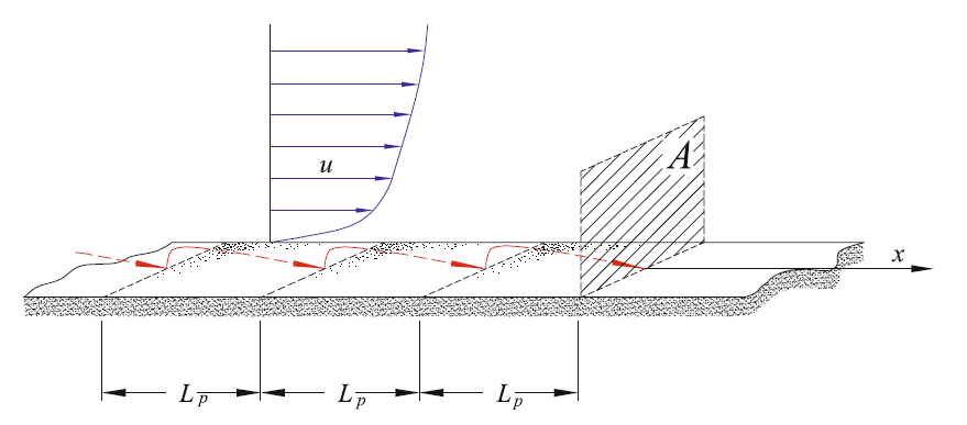
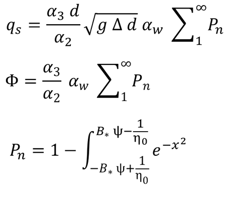
By some assumptions, Einstein calculated solid flow with the probability method, on function of parameters which describe river behavior.
The probability of crossing of section A, is based on water speed and secondment characteristics. Last formula calculates the probability Pn thought assess the solid flow.
Last consideration about Einstein model is about heterogeneity of solid material.
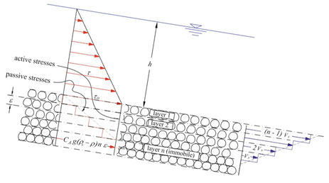
With Coulombian Deterministic Approach there is a bed stratification from the bottom to depth of the solid material.
Du Boys include some hypothesis:
- coulombian friction,
- layer motion of solids,
- n layers with same thick,
- quasi-horizontal found.
Through this analysis, it is possible to define a dimensionless solid flow with the friction relationship between first coulombian layer and last bottom layer.
By that expression is birth Meyer-Peter & Muller empirical formulas and the others studies.
The transport in suspension
To explain the transport in suspension, it is necessary to fix two important conditions:
- the water speed would be bigger then solid speed;
- the flux would be on turbulence condition.
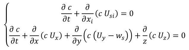
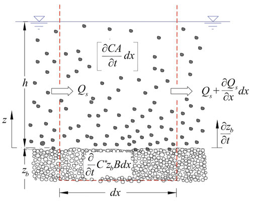
Therefore we have to analyse balance equations, about mass and energy in three directions (x,y,z). Thanks Reynolds system of average, it will possible to determine the Boussinesq dissemination model and introduce epsilon parameter. In fact, on right page, we can see the balance equations and a scheme of Boussinesq model, to understand the mass conservation.
Then will be necessary to introduce two boundary conditions:
- a bidimensional motion in water course;
- homogeneous and stationary field.
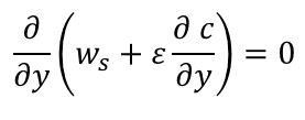
Next formula (under the picture) can explain the balance between dropping and dissemination of solid materials.
Now it is possible to define the problem in two different way, with the assessment of concentration c of the formula:
- Rouse assessment;
- Lane assessment.
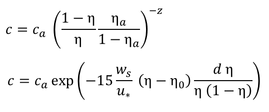
Rouse hypothesizes a logarithmic law for the assumption of turbulence motion and found him formula of concentration. In the same moment Lane defined epsilon and found him exponential formula on function of depth relation (y/h). Next formulas are the relative expressions of Rouse and Lane about concentration issue, but now it will be necessary to explain Ca term.
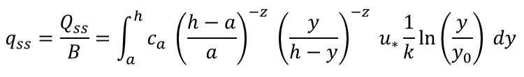
Last expression is about solid suspension linear flow, with two terms: in the integral we have the function of Ca on the depth and the assumption of same speed on x and y directions.
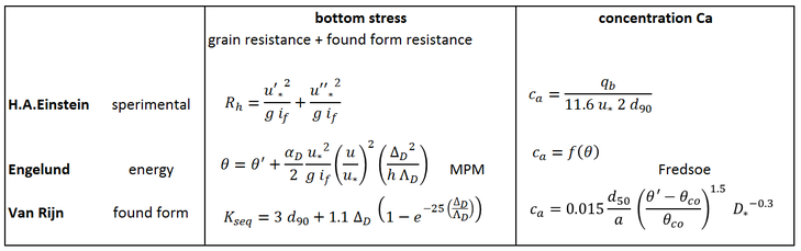
We have got three methods to analyse Ca:
- H. A. Einstein
- Engelund and Fredsoe
- Van Rijn
The first one assumes max concentration on depth a from the bottom; the second puts Ca=F(theta) to connect with the stress moment; the third is about the solid forms and dunes on the bottom.
These methods are from same authors of bottom stress increment criterions.

It is so important define how a dune can move on the bottom.
We talked about different kind of bottom, but there are some difference between dunes and antidunes. Dunes are formed in low speed (Fr<1) behavior and move to downstream, antidunes are formed in high speed (Fr>1) behavior and move to upstream. These effects are caused by a balance of energy: antidunes standing with waves and dunes are opposite the waves, so the erosion-deposit phenomena is opposite and controlled by mass balance.
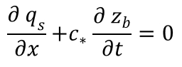
Next expression means that a growth of flow (variation of section) is in equilibrium with an erosion effect on bottom.
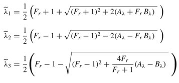
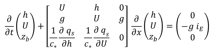
Matrix format and characteristic parameters
Exner study is about erosion effects on the bottom, with the differences between dunes and antidunes.
Thanks to that, it will be known the initial conditions, from upstream and downstream. In fact, it is very important to find where are from the condition to determinate some parameters.
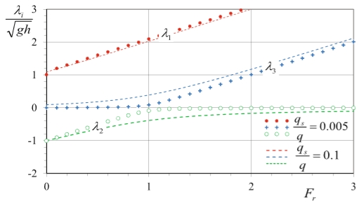
On right of the page we can see the system and matrix formats (1980), which explain solid, liquid and energy balances. Through their we can calculate characteristic lines when all parameters are constant and understand where they are from. There is a big difference between two consideration: if we define a fixed found we calculate three simple parameters on function of Froude number, but if we define a motion found we calculate three equation with others parameters which describe the dunes (or antidunes) motions.
In conclusion, we have got always two information from upstream and one information from downstream, always for every Froud number.
Mathematics models
Hydrodynamic analyses stationary models, but in this case it is not exact. When we speak about mobile found, we can not use stationary models because it does not exist stationary profiles in natural river.
Therefore, we will consider local effects with some hypothesis and simplifications, and can find some difference between fix and mobile found.
Within the limits of the one-dimensional approach, the resulting relations are also suitable to section enlargements. In this case, of course, the variations change sign. In general, the most critical hypothesis of this approach concerns the force against the wall of the transition section. Moreover, independently of the Froude number, we observe erosion and free surface lowering in contractions, but elevation of bed and free surface in enlargements.
If the problem had been faced with a fixed-bed scheme in a mild slope channel, there would have been an upstream backwater profile. On the contrary, the aymptotic solution of the mobile-bed approach does not involve any gradually varied free surface profile, but only a succession of two profiles of uniform flow with discontinuity on the bed and on the free surface through the width change. In practice, however, flood events often have an insufficient duration to the achievement of an equilibrium profile of the bed. An additional phenomenon which tends to further complicate the situation is the non-uniformity of the material, in that the grain size sorting and armoring can further low doen the adjustment process of the bed.
Moreover, it is worth considering also the effect of the secondary circulations, occurring in proximity of width variations, responsible for the formation of bars and pools which, unlike one-dimensional schemes, cause local erosion or deposit values significantly different from the average values.
There will be some approximations to reduce variables in the system, then it will be possible to detect this phenomena through three different mathematics models, as waves study.
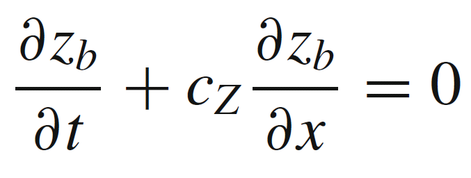
For the simple wave model it is neglected the term if in the first equation of the system, and thus coinciding with the third characteristic calculated by De Vries on matrix method.
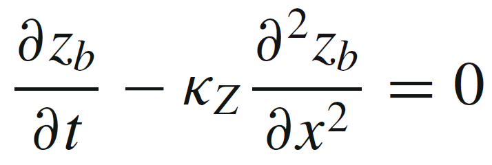
For the parabolic model is hypothesized that the flow can be considered as locally uniform, which is less restrictive than the hypothesis on the simple wave model. This model gives reliable results only for elevated values of x and t. In particular, the time dependence of the discharge can be inserted in the diffusion coefficient Kz.
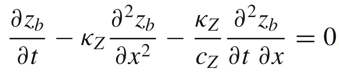
In addition, it can obtain a complete hyperbolic model by combining the hypothesis of the two models previously described.
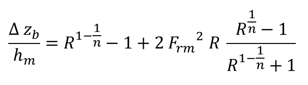
We will study a case of contraction section with parameter R=Bm/Bv>1.
There is an erosion effect on bottom (zb) calculated with next formula:
Fluvial defense works
The defense works are classified in transversal and longitudinal.
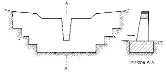
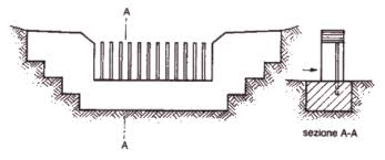
Some famous work used in all the word are the weirs, namely a structure which close the flow way from mountain torrents and rivers. A wire can be close (on the left) or open (some kind on the right):
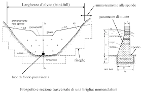
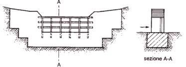
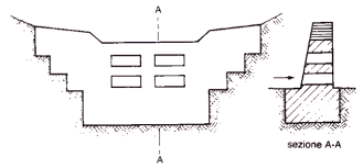


Normally, it is used a set of weirs with a specific distance between; that zone is named deposit place and it can be eroded or reinforced by a concrete layer. In a big deposit place we can found a close weir in enter section and a open weir in exit section. It due to best working of defense system, with the effect of reduction of maximum flow of mod or flood.
The objectives of weir are:
- consolidation, when it is calculated how many weirs have to build for best inclination that avoids erosion and deposit;
- detaining, when it is known the intensity of flow and calculate the inclination for detaining the flood.
Historical function of open weir was granulometry selection, that is the reduction of grain size which compose the flood. Recently, the main problem of blockage of weir was solved with a new system of design of work: it assumes the function of hydrodynamic sieve, therefore it considers the deposit in upstream side, with an energy balance between upstream and its crack.
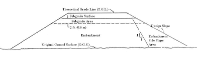
Along largest rivers it can found some built as hills near its banks. These are named embankment and it is used to defend large areas near a river with much flow.
Normally, embankments are made in ground, with some techniques to avoid filtration of water, as concrete blocks or drainage systems.
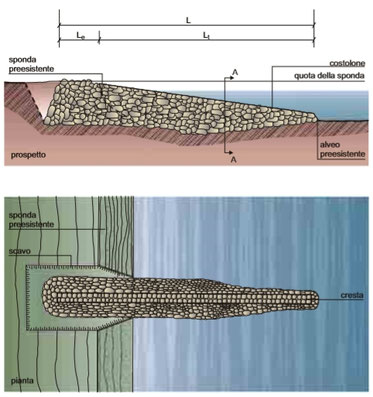
Somewhere it is possible to see builds as cliffs, these are Panels which can avoid erosion of banks and regulate navigation in big rivers.
They are built in rocks or gambion stones or reinforced concrete. Usually they are built on series and symmetrically respect the river, but it very difficult the designing on turn of river because it should be warning to erosion effects.
We can see different kind of panels by the materials and by the form: for example they can be rectangular, circular or asymmetric.
Panels can be swamped or emerged due to water effect and orientation respect the river. Finally, it is important to consider vegetation elements for growth of life on a panel or in the river; it is easy to see several kind of plants and animals which live in both sides.